Introduction to spatial regression

Week 6 - spatial regression

You now have the skills to:

map spatial data
obtain, generate and manipulate raster data
conduct spatial interpolation
identify clustering

This week, and in coming weeks, we are going to start putting these concepts together as part of regression analyses. Regression analyses allow us to look for associations between our outcome of interest (e.g. prevalence of infection, incidence of disease etc.) and a set of predictors.

Univariate Linear Model

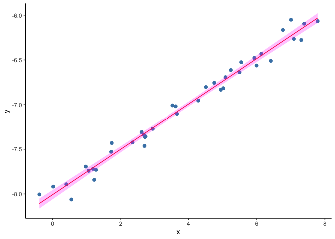
As a first step we will do a recap on a linear regression model. In this problem we have a set of measurments of two variables, say (X) and (Y), and we try to explain the values of our continuous outcome (Y) based on the values on (X). To do this we find the line that is the closest to all the points ((x, y)).

Besides the code displayed here, we will use some additional code to generate some toy datasets that will help illustrate the exposition. Before starting we will load these code as well as the other required libraries, including ggplot2 which will be used for creating most of the images displayed.

library(ggplot2)
library(raster)

## Loading required package: sp

library(ModelMetrics)

## 
## Attaching package: 'ModelMetrics'

## The following object is masked from 'package:base':
## 
##     kappa

library(spaMM)

## spaMM (version 3.0.0) is loaded.
## Type 'help(spaMM)' for a short introduction,
## and news(package='spaMM') for news.

source("https://raw.githubusercontent.com/HughSt/HughSt.github.io/master/course_materials/week6/Lab_files/R%20Files/background_functions.R")

The command below generates a toy dataset that we will use as an example.

# Generate example data
dset1 <- univariate_lm()

# Show data
head(dset1)

##             x         y
## 1 -0.38813740 -8.005137
## 2  0.01616137 -7.917746
## 3  0.40175907 -7.892104
## 4  0.54888497 -8.061714
## 5  0.97495187 -7.694279
## 6  1.05565842 -7.741698

In R we can fit a linear model and make predictions with the comands shown next.

# Fit linear model on dataset 1
m1 <- lm(y ~ x, data = dset1)
m1_pred <- predict(m1, newdata = dset1, interval = "confidence")
dset1$y_hat <- m1_pred[,1]
dset1$y_lwr <- m1_pred[,2]
dset1$y_upr <- m1_pred[,3]

# plot
ggplot(data=dset1, aes(x, y)) + 
  geom_point(col="steelblue", size=2) + 
  geom_line(aes(x, y_hat), col="red") +
  geom_ribbon(aes(ymin=y_lwr, ymax=y_upr), fill="magenta", alpha=.25) +
  theme(panel.grid.major = element_blank(), panel.grid.minor = element_blank(), 
        panel.background = element_blank(), axis.line = element_line(colour = "black"))

Univariate GLM

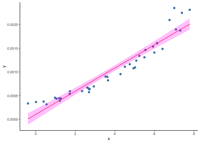
While very useful, it is common that the model above turns out to be a not good assumption. Think of the case where (Y) is constrained to be positive. A straight line, unless it is horizontal, will cross the (y)-axis at some point. If the values of (X) where (Y) becomes negative are rare or they are a set of values we are not interested in, we may simply ignore them, however there are scenarios where we cannot afford having impossible values for (Y).

As an example, we will load a second toy dataset where the outcome (Y) is prevalence of infection (expressed as a probability) and fit a liner regression model. Look at the bottom left corner of figure below. The predictions of (Y) are starting to cross the zero value and become negative, but the observed data remain positive.

# Fit linear model on dataset 2
dset2 <- univariate_glm()
m2 <- lm(y ~ x, data = dset2)
m2_pred <- predict(m2, newdata = dset1, interval = "confidence")
dset2$y_hat <- m2_pred[,1]
dset2$y_lwr <- m2_pred[,2]
dset2$y_upr <- m2_pred[,3]

ggplot(data=subset(dset2), aes(x, y)) + 
  geom_point(col="steelblue", size=2) + 
  geom_line(aes(x, y_hat), col="red") +
  geom_ribbon(aes(ymin=y_lwr, ymax=y_upr), fill="magenta", alpha=.25) +
  theme(panel.grid.major = element_blank(), panel.grid.minor = element_blank(), 
        panel.background = element_blank(), axis.line = element_line(colour = "black"))

A solution to this problem is to use generalized linear models (GLM). A GLM uses a transformation on (Y) where the assumptions of the standard linear regression are valid (figure below), then it goes back to the original scale of (Y) and makes predictions. For example, as our outcome is a probability, we can use the common ‘logit’ transformation, also known as log odds, calculated as log(p/(1-p)) where p is the probability of infection.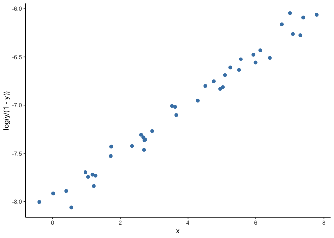

When fitting a GLM to the dataset shown in the second example above, the resulting predictions draw a curve that never reaches zero.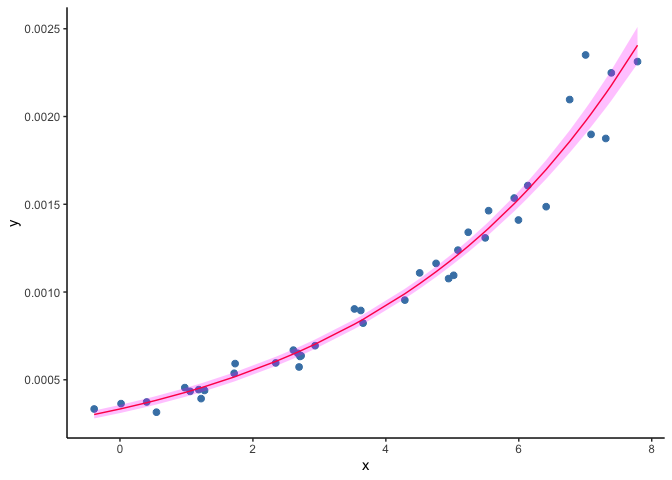

Similarly, we can use the GLM framework to model other non-continuous outcomes. These include binary outcomes (i.e. 0 and 1), multi-class outcomes (e.g. ‘A’, ‘B’ and ‘C’) and counts (e.g. numbers of cases). Here we are going to do a deep dive on binary and counts outcomes as these are likely to be the most common types of outcomes you will deal with.

For the binary case, we are going to use the Ethiopia malaria data. While the outcome of interest here is prevalence, prevalence is just an aggregate of the numbers of 1s and 0s at each location. In this instance we can use what’s called a logistic regression as our data are binomial (numbers positive out of a number examined). Logistic regression works with the logit transformation.

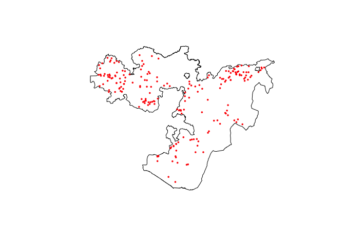
As a reminder, this survey data contains information about number of positive cases and number of examined people in different schools. Spatial information is encoded in the fields longitude and latitude.

# Load data
ETH_malaria_data <- read.csv("https://raw.githubusercontent.com/HughSt/HughSt.github.io/master/course_materials/week1/Lab_files/Data/mal_data_eth_2009_no_dups.csv", header=T) # Case data
ETH_Adm_1 <- raster::getData("GADM", country="ETH", level=1) # Admin boundaries
Oromia <- subset(ETH_Adm_1, NAME_1=="Oromia")
# Plot both country and data points
raster::plot(Oromia)
points(ETH_malaria_data$longitude, ETH_malaria_data$latitude,
       pch = 16, ylab = "Latitude", xlab="Longitude", col="red", cex=.5)

To model and predict malaria prevalence across Oromia State, we need to first obtain predictors as rasters at a common resolution/extent. In this example, we are going to use two of the Bioclim layers, accessible using the getData function in the raster package.

bioclim_layers <- raster::getData('worldclim', var='bio', res=0.5, lon=38.7578, lat=8.9806) # lng/lat for Addis Ababa

We can crop these layers to make them a little easier to handle

bioclim_layers_oromia <- crop(bioclim_layers, Oromia)
plot(bioclim_layers_oromia[[1]]) # Bio1 - Annual mean temperature
lines(Oromia)

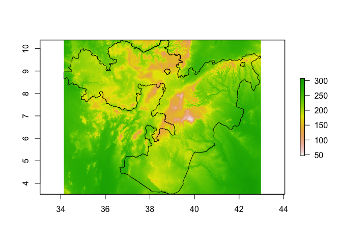
Now let’s extract Bio1 (Annual mean temperature) and Bio2 (Mean Diurnal Range (Mean of monthly (max temp - min temp))) at the observation points

ETH_malaria_data$bioclim1 <- extract(bioclim_layers_oromia[[1]], ETH_malaria_data[,c("longitude", "latitude")])
ETH_malaria_data$bioclim2 <- extract(bioclim_layers_oromia[[2]], ETH_malaria_data[,c("longitude", "latitude")])

Now we fit the model. In the binomial case, it is possible to have a 2 columned matrix as the outcome representing numbers positive and numbers negative. Our outcome could also be a set of 0s and 1s if we had individual level data.

glm_mod_1 <- glm(cbind(pf_pos, examined - pf_pos) ~ bioclim1 + bioclim2, data=ETH_malaria_data, family=binomial())

Now let’s take a look at the model output:

summary(glm_mod_1)

## 
## Call:
## glm(formula = cbind(pf_pos, examined - pf_pos) ~ bioclim1 + bioclim2, 
##     family = binomial(), data = ETH_malaria_data)
## 
## Deviance Residuals: 
##     Min       1Q   Median       3Q      Max  
## -1.4327  -0.9205  -0.7473  -0.5879   7.6321  
## 
## Coefficients:
##               Estimate Std. Error z value Pr(>|z|)    
## (Intercept) -13.717021   2.189372  -6.265 3.72e-10 ***
## bioclim1      0.008466   0.006164   1.374 0.169577    
## bioclim2      0.044857   0.012550   3.574 0.000351 ***
## ---
## Signif. codes:  0 '***' 0.001 '**' 0.01 '*' 0.05 '.' 0.1 ' ' 1
## 
## (Dispersion parameter for binomial family taken to be 1)
## 
##     Null deviance: 383.42  on 202  degrees of freedom
## Residual deviance: 368.12  on 200  degrees of freedom
## AIC: 444.27
## 
## Number of Fisher Scoring iterations: 6

The Deviance Residuals: shows us the variation in how far away our observations are from the predicted values. Observations with a deviance residual in excess of two may indicate lack of fit.

The Coefficients show us the slope of the line fit for each predictor which tells us something about the direction of the association. Positive coefficients suggest a positive relationship and negative a negative relationship. These are all expressed on the log scale as we are working in logit space. The standard error and z values are used to calculate the p-value which tells us how likely this relationship was observed by chance. If you want to express your coefficients as odds ratios, you can exponentiate these values. E.g. the estimate for bioclim 1 is is 0.008466 which is an odds ratio of 1.009.

The Null deviance tells us how well a model only with the intercept (i.e. if you assume the mean at every location) fits the data. Residual deviance tells us how well the model with the predictors fits the data. Lower values (i.e. less deviation of the predicted value from the observed) is better.

In this case, it looks like there is no evidence that bioclim1 is related to prevalence but bioclim2 is. Let’s try re-running the model without bioclim 1.

glm_mod_2 <- glm(cbind(pf_pos, examined - pf_pos) ~ bioclim2, data=ETH_malaria_data, family=binomial())
summary(glm_mod_2)

## 
## Call:
## glm(formula = cbind(pf_pos, examined - pf_pos) ~ bioclim2, family = binomial(), 
##     data = ETH_malaria_data)
## 
## Deviance Residuals: 
##     Min       1Q   Median       3Q      Max  
## -1.3321  -0.9212  -0.7507  -0.6068   7.5499  
## 
## Coefficients:
##              Estimate Std. Error z value Pr(>|z|)    
## (Intercept) -11.97128    1.78167  -6.719 1.83e-11 ***
## bioclim2      0.04455    0.01254   3.554 0.000379 ***
## ---
## Signif. codes:  0 '***' 0.001 '**' 0.01 '*' 0.05 '.' 0.1 ' ' 1
## 
## (Dispersion parameter for binomial family taken to be 1)
## 
##     Null deviance: 383.42  on 202  degrees of freedom
## Residual deviance: 369.98  on 201  degrees of freedom
## AIC: 444.12
## 
## Number of Fisher Scoring iterations: 6

OK the estimate for bioclim2 is 0.04455 which is an odds ratio of 1.05. This means that for every unit increase in mean diurnal range, the odds of infection increase by 5%.

It is possible to explore associations with other sensible covariates in the same way, i.e. by including them in the model and seeing which are ‘significant’. This kind of forward stepwise method to select variables is only 1 way to build a model. Some advocate using AIC or cross-validation techniques which we will introduce later.

It is also useful to check how well your fitted values (i.e. predictions at your data points) line up with the observations.

ggplot() + geom_point(aes(glm_mod_2$fitted, ETH_malaria_data$pf_pr))

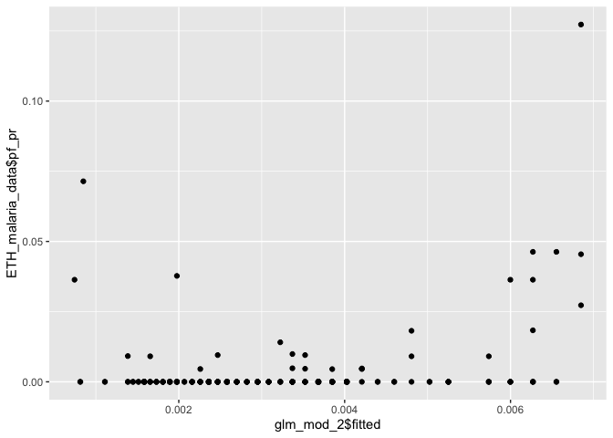
Our fitted values don’t line up particularly well with the observed data, suggesting that bioclim2 alone doesn’t explain prevalence very well.

Once you have a final model you are happy with, it is now possible to predict prevalence at all other locations using the model covariates. In this case, we have a model with only bioclim2. Let’s assume this is our final model and make predictions using this variable.

As we only have 1 covariate, there is no need to worry about resampling rasters. If you are using multiple covariates, you should ensure these are resampled to the same grid (extent and resolution) before extracting and modeling. As a reminder, here is a walkthrough of resmapling.

If you want to predict using a model, you have to provide a data.frame of observations (points) with the same variables used in the model. If you want to produce a risk map, i.e. predict prevalence over a grid, instead of providing a data.frame, the raster package allows you to predict using a model and a raster (layer or stack if multiple layers). Let’s try both.

# Make a prediction at a single location
# with a bioclim2 value of 120
prediction_point <- data.frame(bioclim2 = 120)

# Now predict. Using type='response' tells R you want 
# predictions on the probability scale instead of 
# log odds
predict(glm_mod_2, prediction_point,  type="response")

##          1 
## 0.00132496

# Now let's predict over the whole raster. We first have to 
# make sure that the raster layer(s) pf the covariates
# we want to use to predict have the same name
# as that used in the model (i.e. 'bioclim2')
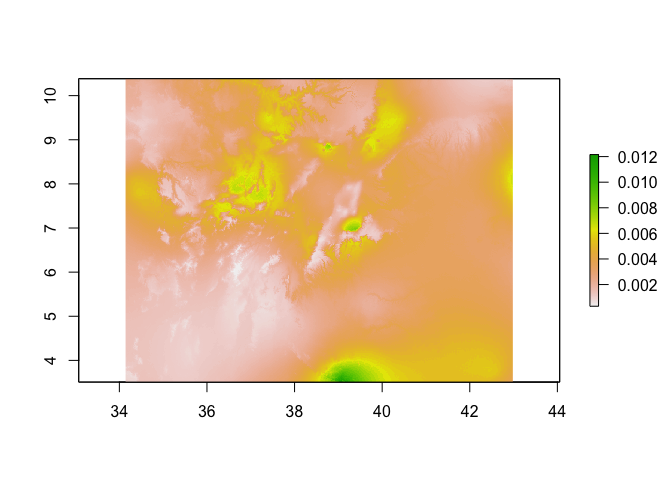
pred_raster <- bioclim_layers_oromia[[2]]
names(pred_raster) <- 'bioclim2'

# Now as we are predicting using a raster, we specify the
# raster first, then the model
predicted_risk <- predict(pred_raster,
                          glm_mod_2,
                          type='response')

# Now plot
plot(predicted_risk)

# or masked to Oromia
predicted_risk_masked <- mask(predicted_risk, Oromia)
plot(predicted_risk_masked)

One of the assumptions we make when fitting GLMs is that the residuals of the model (i.e. what isn’t explained by the covairates) are independent. Often, however, with spatial data this assumption isn’t met. Neighboring values are often correlated with each other. This raises 2 questions:

1) How do you know whether there is any residual spatial autocorrelation?

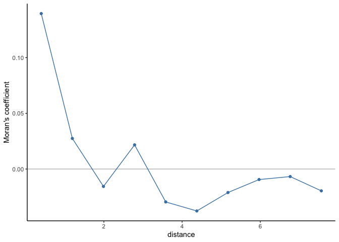
If there is no residual spatial autocorrelation, then we can trust the regression estimates. To test whether the residuals are independent, we can use Moran’s coefficient (as introduced in Week 4. The table and spatial autocorrelogram below suggest that there is spatial autocorrelation up to scales of ~1.2 decimal degress and therefore that the residuals are not independent.

# Compute correlogram of the residuals
nbc <- 10
cor_r <- pgirmess::correlog(coords=ETH_malaria_data[,c("longitude", "latitude")],
                            z=glm_mod_2$residuals,
                            method="Moran", nbclass=nbc)

cor_r

## Moran I statistic 
##       dist.class         coef      p.value    n
##  [1,]  0.3979675  0.139537758 1.452043e-14 3904
##  [2,]  1.1937029  0.027455904 1.132424e-02 5192
##  [3,]  1.9894379 -0.015590957 7.771255e-01 5680
##  [4,]  2.7851728  0.021688238 4.436913e-02 4976
##  [5,]  3.5809077 -0.029494019 9.462506e-01 5078
##  [6,]  4.3766427 -0.037610752 9.943232e-01 5896
##  [7,]  5.1723776 -0.021069731 8.480308e-01 4890
##  [8,]  5.9681126 -0.009427237 5.663123e-01 3694
##  [9,]  6.7638475 -0.006745678 4.501948e-01 1412
## [10,]  7.5595825 -0.019553283 4.527890e-01  284

correlograms <- as.data.frame(cor_r)
correlograms$variable <- "residuals_glm" 

# Plot correlogram
ggplot(subset(correlograms, variable=="residuals_glm"), aes(dist.class, coef)) + 
  geom_hline(yintercept = 0, col="grey") +
  geom_line(col="steelblue") + 
  geom_point(col="steelblue") +
  xlab("distance") + 
  ylab("Moran's coefficient")+
  theme(panel.grid.major = element_blank(), panel.grid.minor = element_blank(), 
        panel.background = element_blank(), axis.line = element_line(colour = "black"))

OK, so we’ve established that our model violates the assumptions of a GLM. This leads to the next question

2) If residual spatial autocorrelation is present, what can we do about it?

As introduced in Week 3, the core idea behind Spatial Statistics is to understand and characterize this spatial dependence that is observed in different processes, for example: amount of rainfall, global temperature, air pollution, etc. Spatial Statistics deal with problems where neighbouring values are expected to be more alike than things further apart from each other.

When we want to measure how much two variables change together, we use the covariance function. Covariance functions are effectively the same as the variogram models you explored in Week 3 and are used to estimate the similarity between values in space as a function of the distance between them. Under the right assumptions, we can also use the covariance function to describe the similarity of the observed values based on their location.

A covariance function K : 𝕊 × 𝕊 → ℝ maps a pair of points z₁ = (s_[1, 1], s_[1, 2]) and z₂ = (s_[2, 1], s_[2, 2]) to the real line. We can define such a function in terms of the distance between a pair of points. Let the distance between the points be given by r = ∥z₁ − z₂∥, the following are examples of covarinace functions:

Exponentiated Quadratic: K(z₁, z₂)=σ²exp(−r²/ρ²)

Rational Quadratic: K(z₁, z₂)=σ²(1 + r²/(2αρ²))^−α

Matern Covariance: K(z₁, z₂)=σ²2^1 − ν/Γ(ν)((2ν)^.5r/ρ)^ν𝒦_ν((2ν)^.5r/ρ)

Here, nu (ν) represents the ‘smoothness’ parameter, alpha α determines the relative weighting of large-scale and small-scale variations, rho (ρ) the scale parameter, Γ is the gamma function and 𝒦_ν is the modified Bessel function of second kind. In the three cases, while less clear in the Matern case, the covariance decreases asymptotically towards zero the larger the value of r. This means that the more distance between a pair of points, the weaker the covariance between them.

The election of which covariance function to use depends on our assumptions about the change in the association between the points across space (eg., the speed of decay).

Geostatistics

Now that we have discussed how the covariance function can help model spatial dependence, we can discuss how to incorporate this ideas into our model. In our GLM example above we fitted a model of the form

η_i = β₀ + β₁x_i + e_i,

Now we will incorporate an spatially correlated random effect (b_i):

η_i = β₀ + β₁x_i + e_i + b_i where spatial correlation is modeled using a covariance function K.

We can implement this model, assuming a Matern covariance, as shown below.

glm_mod_2_spatial <- spaMM::fitme(cbind(pf_pos, examined - pf_pos) ~ bioclim2 + Matern(1|latitude+longitude), data=ETH_malaria_data, family=binomial())
summary(glm_mod_2_spatial)

## formula: cbind(pf_pos, examined - pf_pos) ~ bioclim2 + Matern(1 | latitude + 
##     longitude)
## Estimation of corrPars and lambda by Laplace ML approximation (p_v).
## Estimation of fixed effects by Laplace ML approximation (p_v).
## Estimation of lambda by 'outer' ML, maximizing p_v.
## Family: binomial ( link = logit ) 
##  ------------ Fixed effects (beta) ------------
##             Estimate Cond. SE t-value
## (Intercept) -9.84455  5.61006 -1.7548
## bioclim2     0.01136  0.04051  0.2803
##  --------------- Random effects ---------------
## Family: gaussian ( link = identity ) 
##                    --- Correlation parameters:
##      1.nu     1.rho 
## 0.4695574 2.4472962 
##            --- Variance parameters ('lambda'):
## lambda = var(u) for u ~ Gaussian; 
##    latitude .  :  4.845  
## # of obs: 203; # of groups: latitude ., 203 
##  ------------- Likelihood values  -------------
##                         logLik
## p_v(h) (marginal L): -107.5769

nu (ν) represents the ‘smoothness’ parameter and rho (ρ) the scale parameter. lambda is the estimated variance in the random effect and phi the estimated variance in the residual error.

You can see that the estimate for the effect of bioclim2 has dropped towards 0. While spaMM doesn’t provide p-values, you can calculate the 95% confidence intervals as follows.

coefs <- as.data.frame(summary(glm_mod_2_spatial)$beta_table)

## formula: cbind(pf_pos, examined - pf_pos) ~ bioclim2 + Matern(1 | latitude + 
##     longitude)
## Estimation of corrPars and lambda by Laplace ML approximation (p_v).
## Estimation of fixed effects by Laplace ML approximation (p_v).
## Estimation of lambda by 'outer' ML, maximizing p_v.
## Family: binomial ( link = logit ) 
##  ------------ Fixed effects (beta) ------------
##             Estimate Cond. SE t-value
## (Intercept) -9.84455  5.61006 -1.7548
## bioclim2     0.01136  0.04051  0.2803
##  --------------- Random effects ---------------
## Family: gaussian ( link = identity ) 
##                    --- Correlation parameters:
##      1.nu     1.rho 
## 0.4695574 2.4472962 
##            --- Variance parameters ('lambda'):
## lambda = var(u) for u ~ Gaussian; 
##    latitude .  :  4.845  
## # of obs: 203; # of groups: latitude ., 203 
##  ------------- Likelihood values  -------------
##                         logLik
## p_v(h) (marginal L): -107.5769

row <- row.names(coefs) %in% c('bioclim2')
lower <- coefs[row,'Estimate'] - 1.96*coefs[row, 'Cond. SE']
upper <- coefs[row,'Estimate'] + 1.96*coefs[row, 'Cond. SE']
c(lower, upper)

## [1] -0.06803875  0.09074934

# If you want to express as an odds ratio
OR <- exp(c(lower, upper))

Which shows that having accounted for spatial autocorrelation, there is no evidence that ‘Bioclim2’ is associated with malaria prevalence.

We can also re-test for residual spatial autocorrelation to make sure that this is removed by our spatial model as specified.

# Compute correlogram of the residuals
nbc <- 10
cor_r <- pgirmess::correlog(coords = ETH_malaria_data[,c("longitude", "latitude")],
                            z = residuals(glm_mod_2_spatial),
                            method="Moran", nbclass=nbc)
cor_r

## Moran I statistic 
##       dist.class         coef   p.value    n
##  [1,]  0.3979675 -0.082103557 0.9982340 3904
##  [2,]  1.1937029 -0.004771094 0.4963582 5192
##  [3,]  1.9894379 -0.010640882 0.6170209 5680
##  [4,]  2.7851728  0.005227741 0.3144509 4976
##  [5,]  3.5809077 -0.007276726 0.5446715 5078
##  [6,]  4.3766427  0.007878155 0.2362530 5896
##  [7,]  5.1723776 -0.010644341 0.5983817 4890
##  [8,]  5.9681126  0.010933890 0.2718782 3694
##  [9,]  6.7638475 -0.009638177 0.4949906 1412
## [10,]  7.5595825 -0.007011994 0.3814165  284

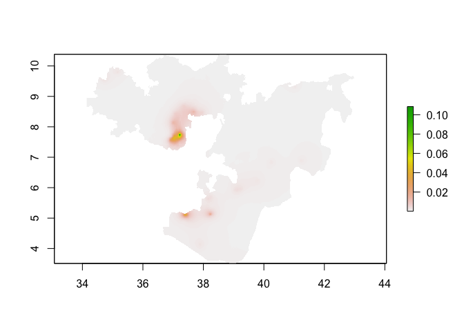
Prediction

Once you have a model that relates our climatic (or other spatial) layers to prevalence, we can predict the probability/prevalence of infection at any location within the region our data are representative where we have values of these climatic layers. For the purpose of demonstration, we are going to assume that bioclim2 is related to prevalence and will therefore be used to make predictions. It is possible to predict from a model directly onto a raster stack of covariates which makes life easy. However, in this case, we are using a geostatistical model, which includes latitude and longitude, and therefore we need to generate rasters of these to add to the stack of bioclim2.

# Create an empty raster with the same extent and resolution as the bioclimatic layers
latitude_raster <- longitude_raster <-raster(nrows = nrow(bioclim_layers_oromia),
                                       ncols = ncol(bioclim_layers_oromia),
                                                    ext = extent(bioclim_layers_oromia))

# Change the values to be latitude and longitude respectively
longitude_raster[] <- coordinates(longitude_raster)[,1]
latitude_raster[] <- coordinates(latitude_raster)[,2]

# Now create a final prediction stack of the 4 variables we need
pred_stack <- stack(bioclim_layers_oromia[[2]],
                    longitude_raster,
                    latitude_raster)

# Rename to ensure the names of the raster layers in the stack match those used in the model
names(pred_stack) <- c("bioclim2", "longitude", "latitude")
plot(pred_stack)

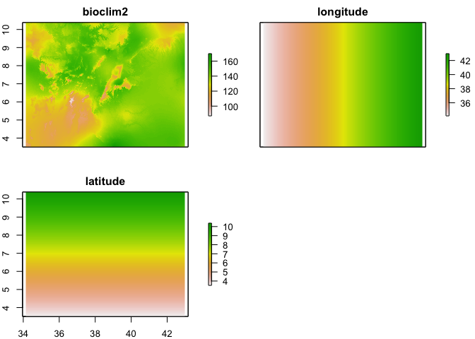
Now we have a stack of rasters of the 4 variables used in the model at the same resolution and extent, we can run the predict function on the stack to produce a raster of preditions.

# Make predictions using the stack of covariates and the model
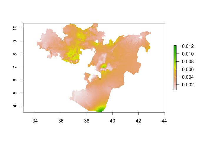
predicted_prevalence_raster <- predict(pred_stack, glm_mod_2_spatial)
plot(predicted_prevalence_raster)
lines(Oromia)

# If you want to clip the predictions to Oromia
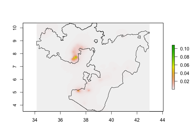
predicted_prevalence_raster_oromia <- mask(predicted_prevalence_raster, Oromia)
plot(predicted_prevalence_raster_oromia)

Model validation

Given that we are interested in building a model in order to make predictions (i.e. a risk map), it is a good idea to validate the model with some independent data. Typically, we do this by removing a fraction of the data (something like 20%) to act as a validation dataset, fitting the model on the remaining 80% and then predicting to the validation set. We can then compare observed versus predicted. If you are being really thorough, you can repeat this process multiple times to make sure every observation has a chance to be in the validation set. This is called v-folds cross-validation. Let’s try the first method.

# take 20% to act as validation set
set.seed(1)
validation_rows <- sample(1:nrow(ETH_malaria_data), 40)
ETH_malaria_data_train <- ETH_malaria_data[-validation_rows,]
ETH_malaria_data_valid <- ETH_malaria_data[validation_rows,]

# Fit model using 80%
glm_mod_2_spatial_validation <- spaMM::fitme(cbind(pf_pos, examined - pf_pos) ~ bioclim2 + Matern(1|latitude+longitude), data=ETH_malaria_data_train, family=binomial())

# PRedict to validation rows and compare
predictions_validation <- predict(glm_mod_2_spatial_validation, ETH_malaria_data_valid)
ggplot() + geom_point(aes(as.vector(predictions_validation), ETH_malaria_data_valid$pf_pr))

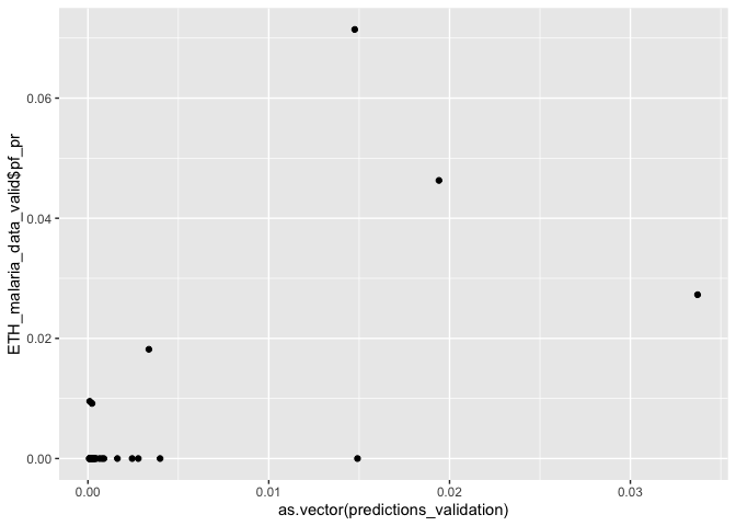
# Calculate mse
mse(predictions_validation, ETH_malaria_data_valid$pf_pr)

## [1] 0.000115546

In this session we learnt the basic concepts of spatial regression. We saw how the spatial covariance is an essential component of a spatial model. By encoding the spatial association into a kernel function, a geostatistic model outperforms linear models even when they include a polynomial representation of the observations coordinates. When properly accounting for the spatial structure of the data, the residuals of the model are independent.

References

Overview of GLMs
Fox (2015) Applied Regression Analysis and Generalized Linear. Chapter 15